
The Journey of RL, Part 2: The Value Hypothesis
Q-Learning and Its Discontents. The compression that made an entire field possible, and the trap it concealed.

In May 1989, a graduate student at King’s College, Cambridge submitted a PhD thesis with the title Learning from Delayed Rewards. The thesis was 241 pages. Its central algorithm had a one-letter name. The letter was Q.
The author was Christopher Watkins, who had been employed as an industrial researcher in southern England for the past four years while completing his thesis. The external examiner on his committee, Andrew Barto, was visiting King’s that spring on sabbatical from the University of Massachusetts. The submission date was forced by the date Barto would fly back to the United States. Watkins’s own account of the timing uses the phrase “by sheer good luck.”
Q-learning did not appear because the field demanded it. It appeared because one mid-career researcher in southern England, who had failed at his first PhD project, who had spent four years writing expert systems at an industrial lab, who had picked up a 1962 textbook in a company library on a hunch, finally saw what the framework he was reading was actually for.
Part 2 begins where Q-learning was born, in a King’s College office in the spring of 1989.
The Letter Was Q
Watkins arrived at King’s College in 1982 as a graduate student. His project was to formalize Jean Piaget’s theory of how intelligence develops in children, with the eventual aim of writing a computer program that would learn the way children do. By his own later assessment, he was “a thoroughly unsuccessful graduate student.” He left without finishing in 1985 and took a job in the AI group at Philips Research Labs in Surrey, England, where he worked on expert systems and decision trees. This was the dominant AI paradigm of the period. The expert systems approach tried to capture human knowledge as explicit rules; the decision tree approach tried to organize those rules into branching decisions. Neither approach asked how the knowledge or the rules were acquired. They started from a body of expertise and tried to encode it.
Watkins kept his interest in the original question. He still hoped to finish a PhD on the genesis of intelligence. The expert systems work was paying the bills.
In 1987 Philips sent him to the Fourth International Workshop on Machine Learning at the University of California, Irvine. He had no paper to present and no specific agenda. During one of the talks he was bored, and he interrupted the speaker to ask a question he later remembered as “totally irrelevant.” The question was whether anyone in the room had done any work on animal learning. The speaker said, without pausing, that all that had been done, and continued his presentation.
Watkins later realized this was wrong in both directions. Animal learning had not all been done. And he had not seen any work in machine learning that built on it. He had given up on children because the problem was too hard. Animals might be tractable.
In the coffee break that followed the session, Richard Sutton came over and introduced himself. Sutton had liked the question. He gave Watkins reprints of several of his recent papers, including a 1983 paper, co-authored with Andrew Barto and Charles Anderson, on a neuronlike system that learned to balance a pole on a cart. Watkins read the pole-balancing paper on the flight back to London, and then again, and then again. He found it highly original, unlike any other work he had seen. It described a small system that learned a difficult control task through direct interaction, getting almost no information about whether any particular action was right, and yet improving. The algorithm seemed to work without obvious theoretical foundation. Watkins felt that there had to be a framework that explained why.
He went to the Philips company library to look for it. The library was small and out of date, which turned out to be useful. The book he found was Applied Dynamic Programming, by Richard Bellman and Stuart Dreyfus, published in 1962. Inside the book was the framework Watkins had been looking for.
Bellman had joined the RAND Corporation in the summer of 1949 and begun working on multistage decision processes. The name “dynamic programming,” which he settled on in the fall of 1950, was, according to the account he later gave in his 1984 autobiography, partly a political maneuver. RAND was funded through the Air Force, and Bellman would write that the Secretary of Defense at the time had a documented hostility to the word “research” and an even sharper hostility to the word “mathematical.” A name was needed that conveyed something serious but did not signal what was actually being done. “Dynamic” suggested time-varying processes; “programming” referred to the planning of multistage operations in the sense of military logistics. The chronology of Bellman’s later account does not quite fit the public record, since his first paper using the term predates the appointment of the Secretary he later blamed. But the broader point survives: the field’s founder did not believe the work could be safely called mathematical research, and the name he chose reflected that belief. By 1957, the year Bellman published the book Dynamic Programming with Princeton University Press, the field had been formalized as the theory of Markov decision processes. The recursive equation at its center, which would later carry his name, said that the value of being in a state was the immediate reward plus the discounted value of the next state, optimized over the available actions.
The 1962 book that Watkins picked up was the applied sequel. It assumed that the structure of the decision process, every transition probability and every reward, was fully known in advance and that the value function could be computed exactly. What Watkins saw, when he closed the book, was the gap. Bellman had given a framework for optimal sequential decisions, but only in the case where the decision-maker already had a complete map. An animal exploring a world does not have a complete map. An animal observes states, chooses actions, receives rewards, finds itself in new states, and starts again.
The question Watkins asked was whether such an animal could learn an optimal policy from experience alone. He worked out, over the next two years, a family of algorithms that could. The simplest of them updated a function he called Q, which assigned to each state-action pair an estimate of the long-run reward of taking that action from that state. The update rule was a single line:
The bracketed term was a temporal-difference error in the sense Sutton had introduced in his 1988 paper. The maximum over next-state actions was new. It made the algorithm capable of learning the optimal policy without ever following it during exploration. This property, which would later be called off-policy learning, would become central to the field and central, eventually, to the field’s later difficulties.
In Spring 1989, by sheer good luck, Andrew Barto arrived at King’s College on sabbatical. Watkins went to see him with an early draft of his thesis. Barto read it and made suggestions; a copy was passed to Sutton, who made more suggestions. Barto agreed to serve as the external examiner on Watkins’s committee, which meant the thesis had to be submitted before he left for the United States. Watkins finished in May. The thesis sketched a proof of convergence for Q-learning but did not prove convergence with probability one. That gap would be closed three years later. In 1992, Peter Dayan, then a graduate student at the Centre for Cognitive Science in Edinburgh, wrote to Watkins to point out that the proof was incomplete. He offered to help fix it. The result was a short joint paper in Machine Learning, titled “Technical Note: Q-Learning,” that proved what the thesis had only sketched.
Q-learning entered the field through a side door. Watkins’s thesis was not published as a book. For several years, American researchers who wanted to read it requested photocopies from Cambridge, which Barto and Sutton mailed out from Amherst. The algorithm that would, two decades later, anchor an entire wave of deep reinforcement learning research entered circulation as a stack of photocopied pages crossing the Atlantic. The algorithm had a one-letter name. The framework it implied would shape what reinforcement learning meant for the next thirty years.
Value as Compression
The Bellman equation in its simplest form said that the value of being in a state is the immediate reward plus the discounted value of the next state, optimized over the available actions:
The equation is recursive. The value of any state is defined in terms of the value of states it leads to. The recursion bottoms out either at terminal states or by the discount factor $\gamma$, which is strictly less than one, ensuring that rewards far in the future contribute less than rewards close at hand. In the more general stochastic case, where transitions are not deterministic, the equation is the same with an expectation over next states. The equation does not solve any specific problem. It only specifies what a solution would have to look like.
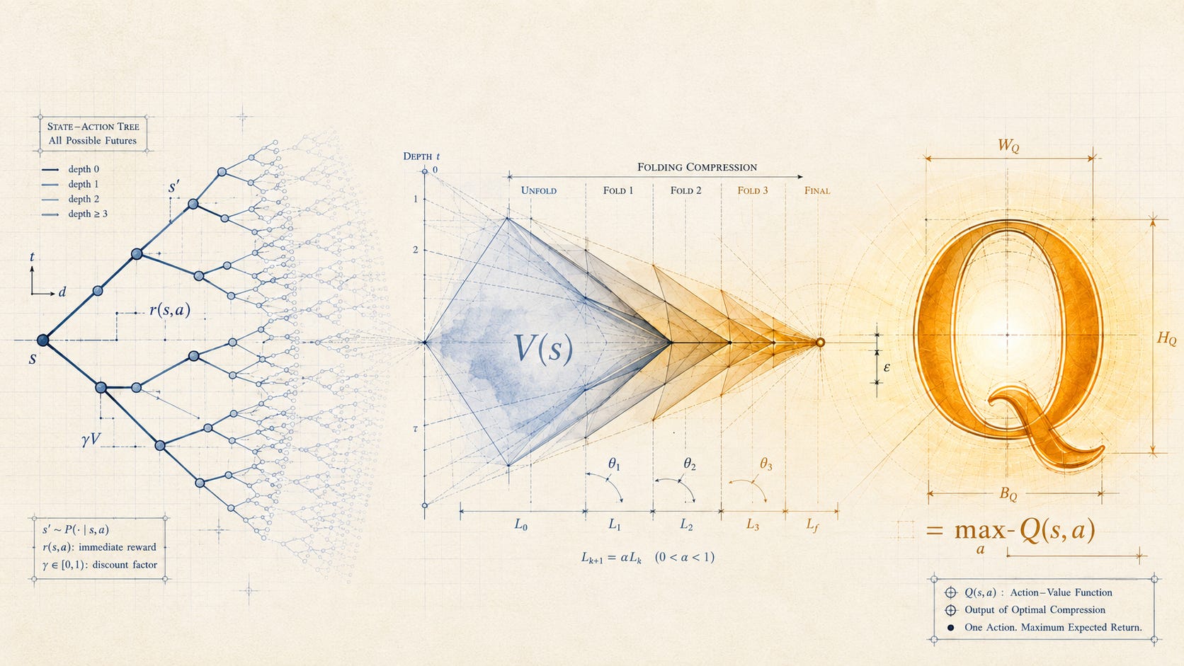
What the equation does, considered as an operation on data, is compression. The whole space of all possible futures from any given state, every trajectory the agent might take, every reward it might collect along the way, is folded into a single number $V(s)$. That number is sufficient, under the Markov assumption, to choose the optimal next action. The agent does not need to remember how it got to the current state, nor does it need to enumerate the futures available from it. It needs the scalar.
This is the second compression in the lineage Part 1 traced. The first was reward itself, the collapse of “goals and purposes” into a single time-indexed scalar quantity. The second was value, the collapse of all reachable futures from a given state into another scalar. The value hypothesis, in the sense Watkins’s thesis introduced it, was the claim that this second compression was tractable. An agent could learn the value function from experience alone, without being given a model of the world, by repeatedly updating its estimate using the temporal-difference error.
The Markov assumption is what makes the compression possible. If the current state contains all the information relevant to predicting the future, then the value function written as $V(s)$ is a sufficient statistic for everything the agent needs to know. Any feature of the agent’s history not summarized in the current state is, by assumption, irrelevant. This is what reinforcement learning shares with thermodynamics and with information theory: the move from a high-dimensional trajectory to a low-dimensional summary is licensed by an assumption about what can be safely forgotten.
When the Markov assumption holds, Bellman’s equation has another useful property. It is a contraction mapping in the space of value functions, which guarantees that iterated application converges to a unique fixed point: the optimal value function $V^*$. Q-learning’s convergence proof, sketched by Watkins in 1989 and completed by Watkins and Dayan in 1992, rests on this property. Each update moves the estimated $Q$ closer to its target. The math works because the assumption holds.
Compression of this kind is a recurring engine across machine learning. The point here is narrower. Watkins’s algorithm, in its 1989 form, depended on two assumptions doing all the load-bearing work: that reward was a well-defined scalar signal from the environment, and that the current state contained all the information needed to predict the future. When both assumptions held, the algorithm worked. The first two decades of reinforcement learning, from the late 1980s to roughly 2010, were spent demonstrating that the algorithm worked in cases where both assumptions held. The next two decades, which Parts 7 through 12 of this series will trace, are about what happens when one of them does not.
The Discontents
In the cases the early Q-learning literature considered, the agent’s state space was small enough to enumerate. A gridworld of a hundred squares, a small Markov decision problem with a few dozen states, a benchmark control task with a discretized angle and velocity: in each of these, the value function could be stored as a table with one entry per state-action pair. Update one entry at a time, sample enough trajectories, and the table converges to the optimal $Q^*$. Watkins and Dayan’s 1992 proof guaranteed it.
The trouble started when the state space grew. Bellman himself had named the problem in 1957, in the same book that formalized dynamic programming: the curse of dimensionality. As the number of state variables increases, the number of distinct states grows exponentially. The number of possible games of chess exceeds the number of atoms in the observable universe. A robot arm with even a few continuous joints has, in any practical sense, infinitely many states. Storing one $Q$ value per state-action pair was not just inefficient. It was not possible.
The standard response was function approximation. Instead of a table, the agent would learn a parametric function, with a manageable number of parameters, that took a state as input and returned an estimate of $Q$. Linear function approximation, where the value was a weighted sum of hand-engineered features of the state, was the obvious starting point and was studied throughout the late 1980s and into the 1990s. Sutton’s 1988 paper on temporal-difference learning had already shown that TD methods could be combined with linear approximators in the on-policy case. The convergence guarantees from the tabular case mostly survived.
The most famous early success of nonlinear function approximation was TD-Gammon, a backgammon program developed by Gerald Tesauro at the IBM Watson Research Center between 1990 and 1998. TD-Gammon trained a multilayer perceptron with eighty hidden units using TD($\lambda$) and self-play, starting from random initial play and playing millions of games against itself. By 1992 it was strong enough to be invited to the World Cup of Backgammon, where in thirty-eight exhibition games against top human players it had a net loss of seven points. By the mid-1990s it was playing at world championship level. The program had been built without expert hand-engineered features and without supervised training on recorded games. The neural network had learned what to value from reward alone.
TD-Gammon was treated, for a long time, as a proof of concept that would surely generalize. It mostly did not. Backgammon has properties that flatter the algorithm. The dice introduce stochasticity that smooths the value landscape and naturally encourages exploration. The game tree is shallow enough that bootstrapping does not accumulate too much error. The state space is large but factored in ways that the network’s hidden units can capture. When researchers tried to repeat the trick in domains without these properties, the algorithms tended to diverge, oscillate, or get stuck. Through the 1990s and 2000s, a recurring observation in the field was that the combination of neural networks, temporal-difference learning, and the off-policy updates Q-learning required was unstable. The exception that TD-Gammon represented did not become the rule researchers had hoped to see.
In 1995, Leemon Baird, then an Air Force officer doing research at the Avionics Directorate of Wright Laboratory at Wright-Patterson Air Force Base in Ohio, presented a paper at the International Conference on Machine Learning that gave the unstable combination its first formal indictment. Baird’s research group at Wright Lab was led by A. Harry Klopf, the same Harry Klopf whose 1972 report had pulled Sutton into reinforcement learning in the first place. Twenty years on, Klopf’s group produced the first formal evidence of where the field’s central algorithm broke. Baird constructed a small example, a Markov decision process with seven states and two actions, in which Q-learning combined with linear function approximation under off-policy sampling provably diverged. The value estimates did not just fail to find the optimum. They grew without bound. The example Baird chose has since been known in the literature as Baird’s counterexample, and it is reproduced in essentially every modern textbook treatment of the topic. What it established was not new in spirit. Researchers had known since the late 1980s that the combination was unstable. What Baird established was that the instability was not an artifact of bad implementation or unfortunate hyperparameters. It was a property of the setting.
The three ingredients Baird identified as jointly responsible were function approximation, bootstrapping, and off-policy learning. Function approximation is what generalizes the value estimate across states. Bootstrapping is what updates the value of one state using the estimated value of another, rather than waiting for actual returns. Off-policy learning is what lets the agent learn about an optimal policy while following a different one for exploration. Each of the three is useful on its own. Each pair of two has been combined successfully in many algorithms. All three together can cause the parameters of the value estimate to escape to infinity.
The name “deadly triad,” which the field would later use for this combination, does not appear in Baird’s 1995 paper. It would not become a fixed term in the literature until Sutton and Barto introduced it in the second edition of their textbook in 2018, after deep reinforcement learning had succeeded despite combining all three. From 1995 to about 2010, however, the underlying observation, that the combination was dangerous in ways that mattered, shaped the field’s choice of methods. The dominant approach was caution: stay tabular where the problem allows, use linear function approximation when generalization is needed, avoid neural networks for the value function, and treat off-policy learning as something to be approached carefully and on-policy alternatives as the safer default.
Through this long period, Q-learning continued to work in the cases it had been designed for. It just did not scale. The algorithm that Watkins had introduced as a way for an agent to learn what to optimize from experience alone, in the most general setting reinforcement learning could imagine, was confined for two decades to settings where the state space could be enumerated or approximated by a handful of linear features. The value hypothesis held in those settings. Outside them, it was not so much that the value hypothesis failed as that the algorithms for testing it broke before the question could be properly posed.
DQN and Its Triumph
The apparatus was repaired by an unexpected route. The 2010s opened with a series of demonstrations that deep convolutional neural networks, trained on large labeled datasets, could solve image classification problems that the field had considered for decades to be far away. The most cited of these was the 2012 ImageNet paper by Krizhevsky, Sutskever, and Hinton, in which a network with sixty million parameters trained on 1.2 million labeled images dropped the top-five error rate on the standard benchmark from twenty-six percent to fifteen. The success was not an incremental improvement on a research curve. It was a step change.
The deep learning revolution was happening in supervised learning, not in reinforcement learning, and there was no obvious reason it should transfer. Q-learning was unstable with neural networks even before the deep learning era. Larger neural networks, naively combined with Q-learning, would on most expectations have made the instability worse. What changed the calculation was a small group of researchers at DeepMind in London who decided to try.
In December 2013, Volodymyr Mnih, Koray Kavukcuoglu, David Silver, Alex Graves, Ioannis Antonoglou, Daan Wierstra, and Martin Riedmiller posted a paper to arXiv with the title “Playing Atari with Deep Reinforcement Learning.” It described a system that took as input the raw pixels of an Atari 2600 game emulator and produced as output a policy for playing the game. The system used a convolutional neural network to estimate the Q function. It was trained by Q-learning. It worked on seven different Atari games. On six of them it outperformed prior reinforcement learning methods. On three of them it surpassed an expert human player.
The 2013 paper was presented at the NeurIPS deep learning workshop and read by a small number of researchers. The result that crystallized the field’s attention was the longer follow-up, published in Nature in February 2015 under the title “Human-level control through deep reinforcement learning,” with a larger team and a much expanded result. The 2015 system was tested on forty-nine Atari games, outperformed the best prior reinforcement learning methods on forty-three of them, and reached a score comparable to a professional human game tester across the full set. The Breakout result became the iconic example: the agent had learned to dig a tunnel along the side of the brick wall, sending the ball behind to destroy blocks more efficiently, a tactic the developers had not anticipated and had not explicitly rewarded.
The 2015 paper added one technical innovation beyond the 2013 system that turned out to matter more than it appeared. Alongside the main Q-network being trained, the algorithm maintained a separate target network whose weights were copied from the main network only periodically, every ten thousand steps in the canonical version. The target used in the temporal-difference update was computed against this slower-moving network, not against the network being currently updated. The change broke the tight feedback loop between the Q-network’s current estimates and the targets it was trying to match, which was one of the three ingredients Baird had identified as jointly dangerous. The combination of function approximation, bootstrapping, and off-policy learning was still present. The target network did not eliminate any of the three. It just kept them from amplifying one another’s errors as quickly.
What DQN had shown was not that the deadly triad had been solved. It was that the deadly triad could be engineered around. Experience replay, the practice of storing past transitions in a buffer and training on randomly sampled batches rather than on the live stream, broke the temporal correlations that gradient methods on neural networks tolerated poorly. The target network broke the self-referential update. Reward clipping bounded the magnitude of the TD error. Each of these was a heuristic. Together they constituted a recipe by which the same combination of ingredients that diverged on Baird’s seven-state counterexample could converge on a multi-million-parameter neural network trained against pixel input from forty-nine Atari games.
The substrate that made all of this possible was the deep network. Q-learning provided the algorithm; deep convolutional networks provided the function class. The convolutional architecture handled the spatial structure of pixel input, where similar shapes recurred at different positions and could share filters. The agent’s value estimate was no longer a table or a linear sum of features. It was a learned hierarchy of representations, computed from raw input. The compression that Bellman had identified, the folding of all future returns into a scalar attached to each state, was now being performed by a network whose internal structure was opaque even to its trainers. The architecture that Rosenblatt had defended at the cost of his career, and that Minsky and Papert had argued in 1969 could not learn certain functions, turned out to be the substrate that made Q-learning scale.
By 2015, Q-learning had moved from a one-line update rule in an unpublished Cambridge thesis to the engine of a system that could play forty-nine arcade games at human level from pixel input. The value hypothesis had been vindicated, in the only domain where it could be tested at scale. What happened next would depend on whether the domain extended further than Atari.
What Compression Cost
The value hypothesis as Q-learning had implemented it rested, in the end, on two compressions doing all the work. The first was reward as scalar. The second was value as the recursive compression of all future scalar reward into a single number per state. Both compressions had been borrowed, the first from behaviorist psychology and the second from operations research. Both had been imported into the architecture of an agent and treated as the agent’s foundation. Both had worked.
What DQN had demonstrated was that the value hypothesis could be deployed at scale. What it had not demonstrated, despite the temptation to read the Nature paper that way, was that the assumptions licensing the compression were now safe to ignore. Atari is a particular kind of environment. The reward signal is the score, which is a number printed on the screen by the game itself. The objective is to maximize that number. The reward function is not learned. It is not contested. There is no ambiguity about what the agent is being asked to do.
The forty-nine Atari games shared this property. They were also Markov, or close enough to it that the assumption was harmless. The agent’s pixel input contained the relevant game state. The next state was a function of the current state and the agent’s action, not of the agent’s history. The Markov property held by construction, because the emulator constructed it. They were finite-horizon, or close enough. They had reward signals that were well-defined functions of game state, returned by the emulator without negotiation. They were the cleanest possible setting for the value hypothesis to be tested.
When reinforcement learning moved off Atari and into settings where the cleanness disappeared, the compression that DQN had made deployable started to show its cost. Two things changed. The Markov assumption that had held by construction in Atari no longer held in domains where agent decisions had long-range dependencies, where the world’s state was only partially observable, or where the relevant context lived in the agent’s history rather than in any single state vector. And the reward signal that had been printed on the screen by the emulator was no longer printed on the screen by anything. Language models had to be trained against signals that were proxies for human preferences. Robotic systems had to be trained against rewards that designers shaped by hand, often badly. Recommender systems had to learn what users wanted from clicks that did not reliably reveal it. In each of these, both halves of the assumption that had licensed the compression broke at once.
Q-learning has no way to tell whether the reward signal is real or constructed. It treats whatever signal arrives as the true objective. The value function the network learns compresses futures with respect to that signal. If the signal is right, the compression is right. If the signal is approximately right at training time but diverges from what was actually wanted at test time, the compression has nothing to fall back on. The value function does not know that its scalar input is wrong. It cannot. The information that would distinguish the right scalar from the approximate one was, by the definition of the architecture, the input to the system, not its concern.
Watkins, looking back on this lineage in a later note on the history of the field, wrote that the assumption that learning agents inhabit a Markov decision process and that learning consists of finding an optimal policy “has been dominant in reinforcement learning research since, and perhaps these basic assumptions have not been sufficiently examined.” Watkins’s own concern was with the first half of that pair: the Markov decision process as a model of the world. The crises this series will trace in Parts 7 through 12 extend the concern to the second half: optimization itself, when the thing being optimized is not given by the world but has to be constructed. The remark is more striking for who is making it than for what it says. The author of Q-learning, thirty years after submitting his thesis, was flagging that the framework he had helped establish might not have been the right one for the field’s later questions. The compression had been a tool. It had also been a commitment, in both halves at once. The field had built thirty years of progress on the commitment, and the parts that were about to crack were the parts where the commitment did the most load-bearing work.
Q-learning’s monopoly over the value side of reinforcement learning was, even in the 1990s, never quite complete. A different lineage, traceable to Williams’s 1992 REINFORCE algorithm and to a current that ran parallel to Watkins’s work without intersecting it, had been arguing that an agent could learn what to do without learning to value states at all. The policy could be parameterized directly. The gradient of expected return could be estimated and followed. Through the 1990s and 2000s, this lineage was the minority view. Most of the canonical results came from value methods. Then, in 2015 and 2016, almost the moment DQN had succeeded, the policy methods began to win in domains where DQN could not.
Part 3 begins where Q-learning’s monopoly began to crack, and where the field discovered that the two routes to the same destination were not, as it had assumed, two routes to the same destination.
This is The Journey of RL, a twelve-part journey across reinforcement learning told through one core question: how did machines learn what to optimize?
Part 3 forthcoming.