
The Journey of RL, Part 3: Policy or Value
The Great Schism. Two routes to the same destination, until they were not.

In May 1992, a forty-seven-year-old Northeastern University computer scientist named Ronald Williams published a paper in Machine Learning introducing a class of algorithms he called REINFORCE. The paper described a way for an agent to improve its behavior by following the gradient of expected reward with respect to its own policy parameters. There was no need to estimate a value function. There was no need to know which action was optimal. The agent needed only to know how its current choices affected the reward it received, and then to nudge its parameters in the direction that improved that reward.
The paper appeared in a Machine Learning special issue that Richard Sutton, then at GTE Laboratories in Waltham, Massachusetts, was editing on reinforcement learning. Williams was six years into a professorship at Northeastern. He had spent the previous decade and a half doing other things. From 1983 to 1986 he had been at UC San Diego, in the Parallel Distributed Processing group led by David Rumelhart, where he had co-authored the 1986 Nature paper on backpropagation. That paper had triggered the boom in neural network research that would eventually consume the field. By 1992, Williams had moved on to Northeastern and had decided that learning by gradient might also apply to learning in environments without labels.
What he had found was that an agent did not need a value function to learn an optimal policy. It could learn the policy directly. The paper was technical, less widely cited at the time than Q-learning, and seemed to occupy a parallel track to the value-based methods that were then becoming dominant. For most of the next two decades, the field treated the two routes as essentially equivalent.
They were not equivalent. Part 3 begins where Q-learning’s monopoly began to crack, and where the field discovered that the two routes were not, as it had assumed, two routes to the same destination.
The Schism
Two mathematical traditions, born within three years of each other. Watkins’s Q-learning in 1989, learning value functions and deriving policies from them by selecting the action with the highest estimated value. Williams’s REINFORCE in 1992, learning policies directly without an intervening value estimate. Both made the same assumptions about the environment. Both reduced to the same task: maximize cumulative reward. Both could be derived from the same Markov decision process formalism. The community at the time treated them as essentially two routes to the same destination, two algorithmic choices that would converge to the same optimal behavior given enough data.
The value-function route was the more developed of the two. Bellman’s dynamic programming dated to 1957, and the convergence theory was relatively mature by the time Watkins’s thesis was submitted. Watkins and Dayan had completed the proof of Q-learning’s almost-sure convergence under tabular representations by 1992. The policy gradient route had less theoretical scaffolding. Williams’s 1992 paper proved that the algorithm’s expected weight updates aligned with the gradient of expected reward, but it did not prove convergence to an optimal policy. REINFORCE estimated the gradient by sampling individual trajectories, and the variance of those estimates was high. In small problems with sparse reward, the policy could drift slowly and then suddenly reverse, or fail to improve at all for long stretches.
Through the 1990s, value-based methods remained the dominant published approach. Q-learning, SARSA, and their variants accumulated convergence proofs, applications to small problems, and a textbook tradition that codified them as canonical. Policy gradient methods stayed in a minority track, with notable contributions from Sutton, Singh, Tsitsiklis, Konda, and a handful of others, but no breakout demonstration that would make the broader research community treat policy methods as the central path.
That changed in 1999. Richard Sutton, then at AT&T Shannon Laboratory in Florham Park, New Jersey, along with David McAllester, Satinder Singh, and Yishay Mansour, submitted a paper to NIPS titled “Policy Gradient Methods for Reinforcement Learning with Function Approximation.” The paper proved what came to be known as the policy gradient theorem: that the gradient of expected return with respect to policy parameters could be written in a form suitable for estimation from experience, even when the policy was represented by a function approximator rather than a table. The theorem made policy gradient methods theoretically rigorous in roughly the way Bellman had made value methods theoretically rigorous forty years earlier.
Actor-critic methods, which had existed in various forms since the Barto-Sutton-Anderson pole-balancing paper of 1983 that Part 1 traced, became the natural synthesis. The actor was a parameterized policy that selected actions. The critic was a learned value function used to reduce the variance of the policy gradient estimate. Actor-critic methods used both routes simultaneously: the policy network for choosing actions, the value network for learning what those choices were worth. The variance problem that had limited REINFORCE in isolation could be partly tamed by borrowing the value-function machinery from the other tradition.
By the early 2000s, the field had three distinct algorithmic families: pure value-based methods, pure policy gradient methods, and hybrid actor-critic methods. The differences among them appeared to be matters of engineering preference rather than principled distinctions. Practitioners chose between them based on the structure of the problem, the form of the action space, and the comfort of the implementer with one mathematical formulation or the other. None of the three was thought to be foundationally better than the others. Each had domains where it worked well and domains where it struggled.
Actor-critic also raised a question that the field did not yet take seriously. If the actor and the critic were learning different things at different rates, which was actually driving the agent’s behavior? The policy network changed continuously as the policy gradient updated its weights. The value network changed in response to the temporal-difference error. The two updates were intertwined, and the convergence properties of the joint system were poorly understood. For small problems with smooth reward landscapes, the joint system worked. For larger problems, the question of which network was responsible for what would become a real engineering concern.
The working assumption was that all three families would eventually converge in capability. Both routes optimized the same objective. Both made the same assumptions. Both were limited by the same problems: function approximation instability, exploration difficulty, reward sparsity. The schism between them, the gap that would open when scaling met them, was not visible from inside the tabular and small-network era.
The Mathematical Asymmetry
For most of the period between 1992 and the mid-2010s, value-based methods looked like the more elegant of the two traditions. The reason was theoretical. Q-learning’s update rule could be derived from the Bellman optimality equation, which had a known fixed point and a known convergence theorem. Watkins and Dayan’s 1992 proof established that under tabular representations and standard stochastic approximation conditions, Q-learning converged to the optimal value function with probability one. The proof was elegant. The algorithm was simple. The mathematical scaffolding was forty years deep, going back to Bellman’s 1957 formulation.
Policy gradient methods had none of these properties in equally strong form. The policy gradient theorem of 1999 proved that the gradient of expected return with respect to policy parameters could be written in a form suitable for estimation from experience. But the theorem did not specify how to estimate the gradient with bounded variance, nor did it guarantee convergence to an optimal policy under function approximation. REINFORCE in particular was famous for high variance. The gradient estimate at any single time step depended on the entire trajectory the agent had followed, and trajectories varied enormously in their cumulative return.
The variance problem was not just an inconvenience. It was a structural feature of the method. To estimate the gradient, the agent had to roll out a policy, observe what reward it accumulated, and adjust the policy in proportion to that reward. If the policy was nearly optimal, the agent saw mostly good outcomes and learned little. If the policy was poor, the agent saw mostly bad outcomes and could not distinguish between actions that were merely bad and actions that were catastrophically bad. The signal-to-noise ratio depended on the policy itself, in a way that value methods had managed to sidestep.
For these reasons, when a researcher wanted to start a new project in reinforcement learning during the 1990s and 2000s, the default choice was a value-based method. Q-learning was the textbook starting point. SARSA, fitted Q-iteration, least-squares temporal difference, dynamic programming with function approximation: these accumulated as a coherent toolkit. Policy gradient methods were available, but they required more careful tuning, more samples, and more patience.
Yet underneath the theoretical asymmetry, there was an asymmetry running in the other direction that the field would not notice until much later. Q-learning’s update rule contained a single mathematical operation that turned out to be more consequential than the convergence proofs had suggested. The target value used in each update was computed by taking the maximum over next-state actions. That operation, written as $\max_{a’} Q(s’, a’)$, required the agent to know all available actions and to be able to enumerate them. For small discrete action spaces, this was no problem. For the action spaces that would matter most in the decade after DQN’s success, it would be a structural obstacle that policy gradient methods did not share. The asymmetry that the field cared about was theoretical convergence. The asymmetry that would matter in practice was whether the algorithm could even be written down.
The Continuous Action Problem
DQN was a system designed around a discrete action space. The Atari 2600 emulator presented the agent with eighteen possible joystick and button combinations at every time step. The agent’s task was to pick one of them. The maximum operation in Q-learning’s update was, in this setting, a simple loop over eighteen possibilities, fast enough that it could be performed millions of times per training run without affecting the algorithm’s runtime profile. Discrete action spaces were the friendliest environment that value-based methods could ask for, and Atari delivered them by construction.
The world outside of Atari was not constructed that way. A robotic arm with seven joints does not select an action from a finite menu. It selects a vector of seven joint torques, each of which can take any value within a continuous range. A simulated humanoid trying to walk does not pick from a list of stride patterns. It outputs continuous force commands to dozens of actuated joints. A self-driving car does not choose between “turn left” and “turn right” as discrete options. It selects a continuous steering angle and a continuous throttle. The action space of physical control problems is not just larger than Atari’s. It is structurally different. Enumeration is not slow. Enumeration is impossible.
Q-learning could not be straightforwardly extended to these settings. The maximum operation required enumeration of actions, and continuous spaces have no enumeration. Variants existed that discretized the action space into bins, but discretization scaled badly with dimensionality. A seven-joint arm with ten discretization levels per joint had ten million actions to enumerate at every time step. A twenty-joint humanoid had ten to the twentieth. The problem was not that value methods worked poorly on continuous control. It was that they could not be written down without modifications that defeated their convergence properties.
Policy gradient methods did not have this problem. The policy was a parameterized function that took states as input and produced actions as output. The output could be a continuous vector as easily as a discrete index. The gradient of expected return with respect to the policy parameters was well-defined whether the action space was discrete or continuous, and the algorithm did not require any maximum operation over actions during training. For continuous control, the policy gradient route was not just one option among several. It was, for a time, the only option that could be expressed within the standard RL formalism.
The first major paper to demonstrate this clearly in the deep learning era was published in September 2015. Timothy Lillicrap, Jonathan Hunt, and six co-authors at Google DeepMind in London posted an arXiv preprint titled “Continuous control with deep reinforcement learning.” The paper introduced an algorithm they called Deep Deterministic Policy Gradient, or DDPG. The algorithm combined two ideas. From the value side, it borrowed the architecture of DQN: a deep neural network estimating a Q-function, trained off-policy with experience replay and a target network. From the policy side, it borrowed the deterministic policy gradient theorem that David Silver and co-authors had proven the previous year at ICML 2014. The policy network output a continuous action; the Q-network evaluated it; the policy network was updated by following the gradient of the Q-network’s output with respect to the action.
DDPG worked. The authors demonstrated it on more than twenty simulated physics tasks, including cartpole swing-up, dexterous manipulation, legged locomotion, and car driving. The algorithm robustly solved tasks that pure Q-learning could not even be written down for. It did so with the same network architecture and hyperparameters across tasks, a level of generality that had been rare in continuous control research up to that point.
DDPG also revealed the structure of the problem that would define the next several years. The interesting question was no longer whether value methods or policy methods were better in principle. The interesting question was which algorithmic combinations could absorb the architectural reality of deep neural networks and continuous action spaces without breaking. DQN had shown that value methods could work with deep networks for discrete actions. DDPG had shown that hybrid methods could work for continuous actions. What had not yet been shown, and what the next two years would establish, was that pure policy methods could work better than either.
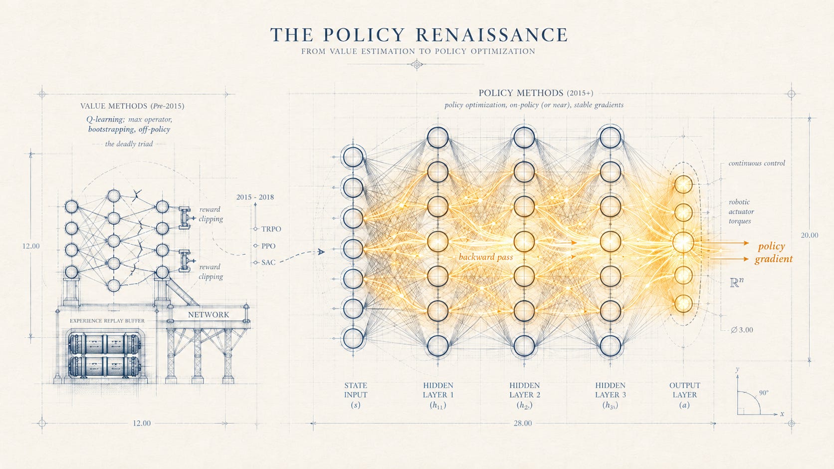
The Policy Renaissance
The cluster of papers that established policy methods as the new mainstream of deep reinforcement learning arrived in a compressed window between February 2015 and July 2017. The first was Trust Region Policy Optimization, posted to arXiv on February 19, 2015, by John Schulman and four co-authors at UC Berkeley. The paper described an iterative procedure for optimizing policies with what the authors called “guaranteed monotonic improvement.” Each policy update was constrained to lie within a trust region around the current policy, defined by a bound on the Kullback-Leibler divergence between the new and old policy distributions. The constraint prevented the catastrophic updates that had plagued earlier policy gradient methods, where a single bad gradient step could destroy weeks of training.
TRPO was theoretically rigorous in a way that earlier policy gradient methods had not been. The trust region constraint had a closed-form derivation, and the paper proved that monotonic improvement was guaranteed when the constraint was satisfied exactly. In practice, satisfying it exactly required solving a constrained optimization problem at every update step, which the authors approximated using conjugate gradient methods on the Fisher information matrix. The approximation worked. TRPO trained neural network policies on robotic locomotion, swimming, hopping, and walking gaits, and on Atari games from raw pixels. It was the first policy gradient method that could be deployed at deep-network scale and trusted not to diverge.
Schulman, the lead author, was at the time a PhD student at Berkeley under Pieter Abbeel. He had also, several months before the TRPO paper appeared, co-founded a research organization called OpenAI. The co-founding was concurrent with his PhD; the TRPO paper carried Berkeley affiliations for all five authors. By the time the next major policy method paper appeared, Schulman had completed his PhD and was working full-time at OpenAI.
The second paper of the cluster was Asynchronous Methods for Deep Reinforcement Learning, presented at the 33rd International Conference on Machine Learning in June 2016. Volodymyr Mnih, who had led the DQN paper at DeepMind, was the lead author. The paper introduced Asynchronous Advantage Actor-Critic, or A3C, which ran multiple parallel agents on separate threads of a single multi-core CPU, each agent collecting its own experience and updating shared network parameters asynchronously. The parallelism let A3C train on Atari games faster than DQN on a GPU, using only commodity CPU hardware. The result was a public demonstration that policy methods could not only match DQN but exceed it in practical training efficiency.
A3C was an actor-critic method, which meant it inherited the value-function machinery from the value-based tradition. The critic network estimated state values; the actor network learned the policy. But the policy was the primary object of optimization, and the value function existed only to reduce variance in the policy gradient estimate. The architectural balance had shifted. Where DQN had been a value method with a deep network attached, A3C was a policy method with a value function as a subordinate component.
The third paper of the cluster, and the one that would prove most consequential, was Proximal Policy Optimization Algorithms, posted to arXiv in July 2017. The lead author was again Schulman, by then at OpenAI, along with four co-authors all at OpenAI: Filip Wolski, Prafulla Dhariwal, Alec Radford, and Oleg Klimov. PPO was a simplification of TRPO. Instead of solving a constrained optimization problem at every step, PPO used a clipped objective function that approximated the trust region constraint with first-order methods. The clipping was a simple operation that any deep learning framework could implement in a few lines of code. The paper claimed that PPO retained “some of the benefits of trust region policy optimization, but they are much simpler to implement, more general, and have better sample complexity empirically.”
PPO became the de facto standard policy gradient algorithm for deep reinforcement learning. Within two years of its publication, it was the default choice for new RL projects in industry, the baseline that new methods had to beat, and the algorithm of choice for the high-profile deployments that would put deep RL on the broader technology-industry map. Among those deployments would be the post-training of large language models, but that story belongs to Part 8.
A fourth paper in the cluster appeared in January 2018, also from Berkeley. Tuomas Haarnoja, Aurick Zhou, Pieter Abbeel, who had been Schulman’s PhD advisor, and Sergey Levine posted Soft Actor-Critic: Off-Policy Maximum Entropy Deep Reinforcement Learning with a Stochastic Actor. SAC combined three threads that had been separately useful. From DDPG it borrowed an off-policy actor-critic architecture with experience replay. From the on-policy methods it borrowed a stochastic policy, so that the agent retained the natural exploration that deterministic policies lacked. From the maximum entropy reinforcement learning literature it borrowed an explicit entropy bonus, which encouraged the policy to remain random where multiple actions were nearly equally good. The entropy bonus acted as a built-in exploration mechanism that did not require tuning a separate exploration schedule. SAC outperformed DDPG and PPO on most continuous control benchmarks, achieved more stable training across random seeds, and required less hyperparameter tuning to do so.
By 2018, the algorithmic landscape of deep reinforcement learning had a clear shape. On-policy policy gradient methods like TRPO, A3C, and PPO covered cases where on-policy data was cheap and stability was the priority. Off-policy actor-critic methods like DDPG and SAC covered cases where sample efficiency mattered and continuous actions had to be controlled. Pure value-based methods like DQN remained competitive on discrete action problems where the maximum operation was easy and the engineering heuristics could be tuned. But the center of gravity had moved. Policy was the primary object of optimization; value functions, when present, served the policy rather than the other way around.
By 2018, the schism between policy and value methods was no longer invisible. TRPO, A3C, DDPG, PPO, and SAC had collectively shown that policy methods, in their various forms, were not just viable at deep-network scale but were often preferable. The two routes had not converged in capability. They had separated.
Survived Contact
The reason policy methods won, in the period that mattered, was not that the policy gradient theorem was more elegant than the Bellman equation. It was that the policy gradient theorem made fewer demands on the network it was being computed through. A policy network outputs an action. The gradient flows backward through a single function. There is no maximum operation, no bootstrapping target, no off-policy update that depends on the network’s own current estimates as a moving target. The deadly triad that Part 2 traced, the combination of function approximation, bootstrapping, and off-policy learning whose instability Baird had formalized in 1995, was not a feature of pure policy gradient methods. The triad did not apply.
Value methods had succeeded with deep networks in DQN, but only by surrounding the core algorithm with engineering heuristics: experience replay, target networks, reward clipping, careful hyperparameter tuning. Each heuristic was an attempt to soften one of the deadly triad’s three ingredients without removing it. The combination worked on Atari, where the action space was discrete, the reward function was clean, and the environment was Markov by construction. The combination worked less well as the field tried to extend it.
To see why the deadly triad was destabilizing for value methods but inert for pure policy methods, it helps to look at what each ingredient does in the update. Function approximation, combined with a learned target, creates a feedback loop in which the network is trained to predict targets that are themselves outputs of the network. Bootstrapping turns this loop into a recursive estimate, where every update changes both the prediction and the target. Off-policy learning means that the distribution of data the network is trained on diverges from the distribution under which the predictions are being evaluated. In combination, the three create a learning dynamic in which small errors can compound rather than dampen. Q-learning was particularly exposed because all three ingredients were structural to the algorithm and could not be removed without changing what the algorithm was. Policy gradient methods used function approximation, but the target of the policy update was a Monte Carlo estimate of return, not a bootstrapped value, and the data distribution was generated on-policy by definition.
Policy gradient methods needed fewer such heuristics. They had their own problems, principally high variance in the gradient estimate, but the problems they had were the kind that scaled well with compute. A high-variance estimator becomes a low-variance estimator when averaged over enough samples, and modern GPUs provided enough samples per second to make the averaging tractable. Variance was a problem the architecture of deep learning was naturally suited to absorb. The deadly triad was not.
Variance was also a problem the engineering culture of deep learning was already equipped to address. The standard tool was batching. If a single gradient estimate had high variance, the average of a large batch had lower variance. GPUs were good at the kind of dense parallel arithmetic that batch averaging required. By the mid-2010s, an industrial RL pipeline could produce hundreds of thousands of policy gradient samples per second, average them, and use the resulting estimate to update the policy. The variance that had limited REINFORCE in the 1990s was no longer a property of the algorithm. It was a property of how much compute was thrown at it. Scaling compute was something the deep learning industry was already learning to do.
This is the sense in which policy methods survived contact with neural networks. Value methods could be made to work with neural networks, given enough engineering. Policy methods worked with neural networks because the gradient flow through a policy network did not require the algorithm to violate the assumptions under which gradient descent is stable. The asymmetry was structural. The field had spent two decades treating the choice between policy and value as a matter of engineering preference, when in fact it was a matter of compatibility with the function approximator that would eventually dominate every domain.
What the two routes had appeared to share, in the tabular and small-network era, was their convergence to the same optimal behavior. They optimized the same objective. They made the same assumptions about the environment. What they did not share, and what the field did not realize until it tried, was their compatibility with the substrate on which they would be deployed. The destination was the same. The terrain to get there was not.
By 2017, the working assumption of the previous twenty years had collapsed. The two routes were not equivalent. One of them had survived the deep learning era largely intact, and the other had survived only with the help of heuristic scaffolding that revealed how fragile the underlying algorithm was. The schism that had been invisible in the 1990s was now the central engineering fact of deep reinforcement learning.
Schulman’s PPO algorithm would, within a few years of its 2017 publication, become the algorithm behind the post-training of large language models. The reinforcement learning from human feedback that produced ChatGPT and its successors used PPO as the optimization engine. The policy was the language model itself; the reward was a learned scalar from a preference model; the gradient flowed through the same trust-region-approximation that Schulman had simplified at OpenAI in 2017. A method that had emerged in the mid-2010s to solve continuous control problems had become, by the early 2020s, the foundation of how machine intelligence learned to talk.
What had happened to the value-function tradition was not that it had been disproved. Q-learning still worked, and its descendants still appeared in published work. What had happened was that the central question reinforcement learning was asking had shifted. For the field’s first three decades, the question was how to learn what to optimize from experience alone. By the late 2010s, that question had been answered well enough to deploy. The new question, which Part 4 turns to, was different. It was not about how an agent learned what to optimize. It was about what was worth measuring in the first place.
This is The Journey of RL, a twelve-part journey across reinforcement learning told through one core question: how did machines learn what to optimize?
Part 4 forthcoming.
Nice history and review of reinforcement learning, showing how the problem space affects which algorithms work when.