

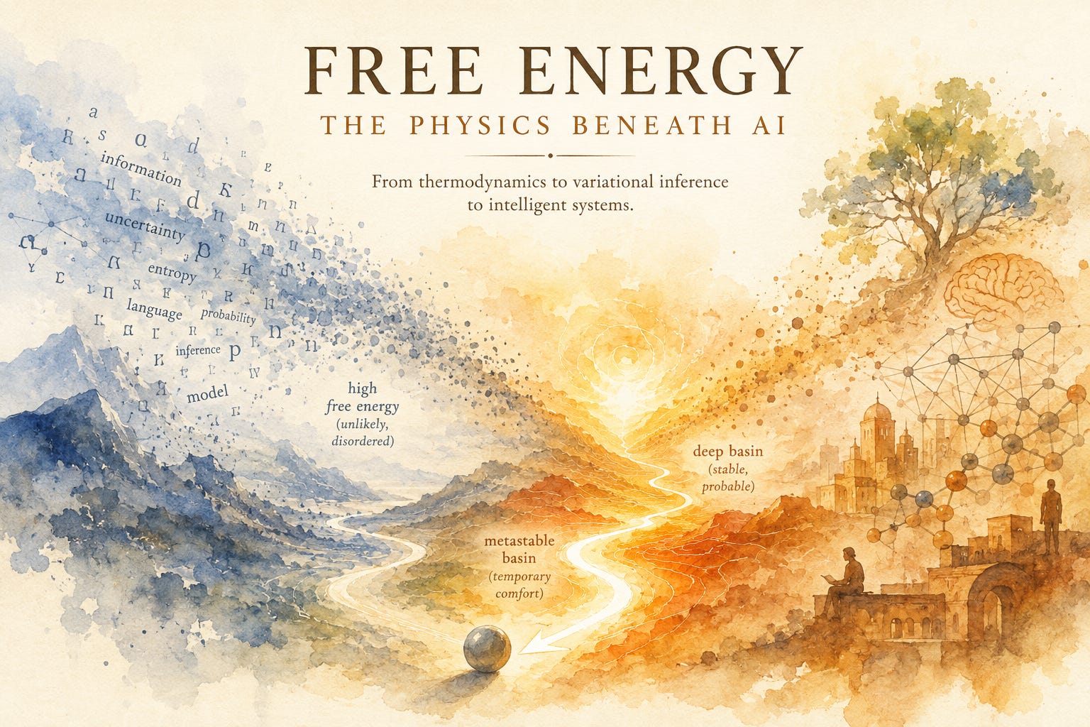
Put a ball on a slope and let go. It moves.
The ball has no model of the valley. It does not calculate a trajectory, enumerate possible destinations, or represent the state toward which it is heading. At every instant, the physics is local. Yet the result looks global: the ball finds lower ground.
This is one of the oldest tricks in nature. A gas relaxes toward equilibrium. A crystal assembles. A protein folds. A chemical reaction proceeds when conditions favor it. Enormous spaces of possible configurations are navigated without anything searching them one by one. None of these systems knows where it is going. What does the work is the shape of the space they move through: a landscape where, from any point, some directions lead down. Local physics is enough to follow them, and free energy is one of the quantities that defines which way down is.
The idea began in nineteenth-century thermodynamics, in the work of Hermann von Helmholtz and Josiah Willard Gibbs. It passed through statistical mechanics, where Ludwig Boltzmann connected energy to probability. Then it appeared again in Bayesian inference, machine learning, energy-based models, variational methods, and theories of biological intelligence.
The equations are not always describing the same physical quantity. That distinction matters. But the computational idea underneath them is remarkably persistent: assign a single number to every possible configuration, turning a difficult global problem into a landscape, then let local dynamics do the search. That may be one of the deepest connections between physics and AI.
Conservation says nothing about direction
Energy is conserved. Use some, and it does not disappear. It changes form.
That makes energy fundamental, but it also creates a problem. If the total amount of energy in an isolated system does not simply vanish, why do physical processes have preferred directions? A hot cup of coffee cools; it does not spontaneously draw heat from the room and become hotter. A gas released into a box spreads out; it does not ordinarily gather itself into one corner again. The total energy can remain the same while the system loses something else: its capacity to produce directed change.
Thermodynamics captures this through free energy. The simplest version, Helmholtz free energy, is written
F = U − TS
where U is the system’s internal energy, which is what the word energy has meant everywhere above: the total energy the system has stored, in molecular motion, in bonds, in interactions between particles. T is temperature and S is entropy.
The reason this quantity matters is that systems move toward lower values of it. Left alone at a fixed temperature, a system settles where F is smallest. That is the sense in which free energy defines which way is down.
Read literally, the formula makes free energy look like a portion of the internal energy: start with U, subtract TS, keep the rest. That is a reasonable working intuition and close to what free means here. The TS term is the part entropy holds back, unavailable for doing work, and the hotter things get the more of it is held.
The size of that deduction depends on temperature, which is a property of the surroundings rather than something stored inside the system. The same system, with exactly the same U, placed somewhere colder, has a different F. So the two quantities answer different questions. U asks how much energy is in there. F asks how much of it the current conditions will let you use.
Entropy is the term that makes this interesting, and what it does is count arrangements. Flip a hundred coins. There is exactly one way for all of them to land heads, and roughly 10^29 ways for exactly half of them to. Nothing pushes the coins toward a fifty-fifty split; no force prefers it. That outcome simply has overwhelmingly more ways of happening, and the counting alone is enough to make it near-certain.
Physical systems work the same way. Entropy counts how many distinct microscopic arrangements produce the same overall state, and the formula shows why that matters. F gets smaller when U is small, and F also gets smaller when S is large. So a state can earn a low free energy in either of two quite different ways: by being low in energy, or by having far more arrangements available. The two routes often pull in opposite directions.
Water and ice are the familiar case. Ice has lower energy, its molecules locked into a lattice by bonds that cost energy to break. Liquid water has vastly higher entropy, since the same molecules can be arranged in an astronomical number of ways while still being water. Which one nature chooses depends on temperature, and the formula says exactly how. When T is small, the TS term barely counts, the low-energy state wins, and water freezes. When T is large, the TS term dominates, the high-multiplicity state wins, and ice melts. At exactly zero degrees Celsius the two terms balance, which is why that is where the change happens.
That is what temperature is doing in the formula. It sets how much the system cares about having options. Minimizing free energy is therefore not the same as minimizing energy, and not the same as maximizing entropy. It is finding where the trade between them settles, given how hot things are. Nature has converted a competition between energy and multiplicity into a landscape.
The landscape does the thinking
Imagine a mountain range. Every possible configuration of a system occupies a point somewhere on the terrain, and height represents free energy. Some regions are peaks. Some are shallow depressions. Some are deep valleys. The system moves through this terrain according to its local dynamics. It does not need to know the coordinates of the deepest valley. It only needs the physics governing what happens where it already is.
This distinction is easy to miss. We often describe optimization as if the optimizer were searching for an answer. But gradient descent does not know the minimum either. It knows only which way is downhill from where it currently stands. The update is local. The consequence can be global.
The difference shows up in what each approach costs. A search has to consider candidates, which means the work grows with how many there are. A descent considers only the neighborhood of wherever it currently sits, which means the work per step is the same whether the space holds a thousand candidates or a number with no name. What grows instead is the number of steps, and that turns out to be a far gentler kind of growth. This is why methods that would be unthinkable as searches are routine as descents.
A neural network may contain billions of parameters, making exhaustive search absurd. Yet training does not inspect every possible setting of those parameters; it constructs a loss landscape and repeatedly makes local moves. Physics discovered this architecture long before machine learning did: do not specify the solution, specify a quantity whose local improvement tends to produce solutions, and let dynamics replace search.
Boltzmann’s bridge
The connection becomes deeper in statistical mechanics. A macroscopic object looks simple: a temperature, a pressure, a volume. Microscopically, however, it may contain an astronomical number of particles, each contributing to an even more astronomical configuration space. There is no practical sense in which nature can enumerate these possibilities, so statistical mechanics describes them probabilistically instead.
Boltzmann’s contribution was to make that probability explicit. The chance of finding a system in some configuration with energy E, at temperature T, is proportional to
p ∝ e^(−E / kT)
where k is Boltzmann’s constant. This rule is called the Boltzmann distribution. Lower-energy configurations come out more likely, and temperature sets how much more. When T is small, even a slight energy advantage makes one configuration overwhelmingly more probable than another. When T is large, the exponent shrinks toward zero for everything, and configurations with very different energies end up nearly equally likely. Temperature is the scale against which energy differences are measured.
This creates a remarkable bridge: energy and probability become two descriptions of the same landscape. Low energy corresponds to high probability, high energy to low probability, and that single equation would later become extremely useful in machine learning.
Energy is the cheaper currency
Energy earns its place in machine learning through a practical asymmetry: turning energies into actual probabilities is expensive, and comparing energies is not. The Boltzmann formula gives a proportionality rather than a probability. To get real numbers that add up to one, each e^(−E/kT) has to be divided by the total of that same quantity across every possible configuration, and computing that total means visiting all of them. Energies carry no such requirement. You can score a single configuration on its own, without reference to any other, and comparing two such scores already tells you which is the more likely.
That total is not a stranger. Take it, take its logarithm, multiply by minus kT, and what comes out is the free energy from the previous section. The quantity that tells a thermodynamic system which way is downhill and the quantity that turns a set of energies into a probability distribution are the same object approached from two directions. Thermodynamics and statistical mechanics meet here.
Scoring configurations by energy rather than probability is the basic intuition behind energy-based models, going back to the Boltzmann machine that Geoffrey Hinton and Terrence Sejnowski built in the mid-1980s on exactly the Boltzmann distribution above, which is where the model takes its name. A configuration here is a piece of data, an image or a pattern, not a setting of the network’s weights.
Instead of asking what probability a configuration should have, the model asks how well it fits the patterns in the data it was trained on. A photograph of a face gets low energy. Random static gets high energy. Training is the process of adjusting the weights until that is true, which means training is what builds the landscape in the first place.
Calling that score an energy rather than simply a score is not decoration. For ranking alone, any fit score would do. What the energy framing keeps in reach is the Boltzmann relation, which converts differences in energy into ratios of probability. Two configurations whose energies differ by about 2.3 units of kT are ten times apart in how likely they are; a gap of seven units puts them a thousand times apart.
An ordinary model that scores one image 0.1 and another 0.3 has said which it prefers and nothing more. It has not said the second is three times as likely, and in general it is not. Those numbers carry an order and no calibrated distance. An energy model has said by how much, on a scale that converts, and that is what makes it possible to sample from the model rather than only rank the things it is handed.
Generating or repairing something afterwards works the other way around. The weights are fixed now, and what moves is the configuration itself: start from some pattern, perhaps a corrupted or half-finished one, and let it slide downhill until it arrives somewhere the model rates as plausible. Learning builds the terrain by adjusting weights; inference walks that terrain with the weights held still.
A model does not need the answer
Suppose an AI observes something but cannot directly see what caused it. The visible data may have been produced by countless hidden states, and Bayesian inference asks which of those states are plausible given what was observed. In simple problems, that question can be answered exactly. In interesting ones, it often cannot: the space of possible explanations becomes too large, and calculating the full distribution over them is itself the impossible problem.
Variational inference, developed through the 1990s by researchers including Geoffrey Hinton, Michael Jordan, and their collaborators, makes a peculiar move. It stops trying to calculate the answer. Instead, it creates a simpler distribution of beliefs that the machine can represent, then gradually changes that distribution until it behaves as much as possible like the inaccessible one. Inference becomes optimization: one pressure forces the belief to explain the observation, another prevents it from becoming needlessly strange, brittle, or detached from what was plausible beforehand. The result is conventionally described using variational free energy.
This is not Helmholtz free energy hiding inside a neural network. The quantities have different meanings. But the mathematical architecture has survived the journey from physics into inference. There is a space of possible states, a single number that ranks them, and a dynamics that moves toward better regions without ever calculating the final answer directly. The belief does not solve for the posterior, the distribution over hidden states that Bayesian inference asks for and cannot afford to compute. It relaxes toward it. A problem that looked like calculation has been converted into motion.
Inference can be relaxation
Normally, we imagine reasoning as the production of an answer: question in, computation happens, answer out. Variational inference suggests another picture. It starts from a guess, some simple distribution the machine can actually write down, a bell curve say, described by nothing more than a center and a width. An objective scores how badly this guess matches the distribution that was actually wanted. Then the center and the width move, a little at a time, in whatever direction lowers that score. The posterior itself never gets computed. The guess creeps toward it and stops when it can improve no further.
This is a surprisingly physical picture of inference. A belief can occupy a bad configuration in much the same abstract sense that a physical system can occupy a high-free-energy configuration. New evidence changes the landscape, the distribution moves, and a new equilibrium becomes preferable. The inference problem has become something a dynamical system can solve.
The same trick appears across AI
Once you see this pattern, it becomes difficult not to see it everywhere.
A neural network is never handed its final weights; training defines an objective and lets optimization discover them. An energy-based model does not list every valid configuration; it learns a surface on which valid configurations lie lower. A Hopfield network, the model John Hopfield introduced in 1982 by way of the same statistical mechanics as the Boltzmann machine, stores memories as attractors: give it a corrupted pattern and its dynamics settle into a nearby basin. A diffusion model begins with noise and repeatedly follows a learned field toward regions compatible with the data distribution. A variational autoencoder does not assign each observation a single hidden explanation; it learns a distribution over latent explanations while balancing reconstruction against a prior.
These systems are technically different, and calling all of them free-energy minimizers would erase important distinctions. But the differences sort themselves along two questions, and asking them turns the list above into something more orderly than a list.
The first question is what moves. For an ordinary classifier during training, the weights move. For classical variational inference, the weights stay put and the parameters of a guessed distribution move instead, a handful of numbers describing a curve. For a Hopfield network completing a memory or a diffusion model denoising an image, neither of those moves: the data itself moves, sliding across a terrain the weights have already fixed in place.
The second question is when. Training-time descent happens once and the result serves every input afterwards. Inference-time descent happens afresh for each new case, and by then the weights are fixed: what descends is whatever the first question named, the parameters of a guess or the data itself. An ordinary classifier and a transformer descend only during training; inference is a single forward pass, one layer after another, with nothing minimized along the way. Energy-based models, Hopfield networks and diffusion models keep descending at inference as well. And a variational autoencoder is the interesting hybrid: it moves the descent that classical variational inference would perform for every observation back into training, learning an encoder that produces the answer in one pass instead. Speed bought with a small loss of accuracy.
What all of them share is an architectural move: a hard global problem is transformed into local dynamics on a designed landscape. This is more general than gradient descent. It is a way of outsourcing computation to geometry.
Local minima are not accidents
Landscapes also explain why systems get stuck. A ball descending a mountain does not necessarily reach the lowest point on Earth; it reaches whatever basin its trajectory allows. Physical systems encounter metastable states, configurations that are locally stable even though lower-free-energy states exist elsewhere. Glass is the classic case: its microscopic structure is trapped away from equilibrium because reaching a better arrangement would require crossing barriers it has no way to cross at room temperature.
Optimization has the same problem. A learning system can settle into a set of weights that is locally good without being globally best, and noise, temperature, initialization, momentum and architecture all influence which barriers get crossed and which basin ends up occupied. This makes the useful question something other than where the minima are. What matters is which trajectories through the landscape are reachable at all. Two systems can share an objective and still learn differently because their dynamics differ, meaning the rule that generates each next step: how far it goes, how much randomness it carries, how much of the previous step it carries forward. The landscape defines possibility. The dynamics define reachability.
When the Ball Picks the Hill
Free energy began as an answer to a physical question: given the constraints, which changes can happen spontaneously? AI keeps rediscovering variations of the same computational move. Do not enumerate every possibility. Do not calculate the global answer directly if you do not have to. Construct a landscape, define what counts as downhill, and let local dynamics perform the computation.
A protein can fold without knowing its final shape. A Bayesian approximation can approach a posterior it cannot calculate. A neural network can find parameters nobody could specify by hand. A world model may eventually allow an agent to navigate futures too numerous to enumerate. The intelligence is not necessarily in knowing the destination. Sometimes it is in having the right terrain.
Every landscape in this article was built by something that was not doing the descending. Physical law and boundary conditions build the thermodynamic one. A person sitting down to write an objective function builds the machine learning one, and everything the system will ever count as progress follows from that decision. The descent is automatic. The choice of terrain is not.
Which is where the analogy runs out. A ball has no opinion about the hill, and no way to act on one if it had. A learning system sits less cleanly apart from its terrain. The landscape it descends is assembled out of an architecture, a body of data and an objective, and each of those is a thing that can itself be searched over, generated, or rewritten.
Systems have started doing the first two. Architecture search selects the shape of the terrain before anything descends it, since the choice of architecture is part of what fixes the geometry. A model trained on its own outputs, as AlphaZero was through self-play, alters the data that shaped the terrain in the first place, so each round of descent changes the ground the next round will run on. Neither of those picks its own objective. Choosing where the bottom should be is a different act from finding it, and no system does the first one yet.
And that leaves AI with a question thermodynamics never had to answer: what happens when the thing doing the descending learns to pick its own objective?
This article paints the wide picture. For a more systematic treatment of these correspondences, one at a time, see The Thermodynamics of Intelligence, a nine-part series examining exactly how far each one holds.
What if synchronization is the default? One big wave is more efficient than many small waves. Everything on the same wavelength, functioning as one. Which qualifies as order.
So the energy is captured, coalesced. Lasers are synchronized light waves.
Signal, while the free energy is noise. Though it equilibrates.
The node is synchronization. The network is harmonization.
https://www.quantamagazine.org/physicists-discover-exotic-patterns-of-synchronization-20190404/
You beautifully distinguish between cognition and descent. Human reasoning is coherence‑driven; we preserve our identity across time, context, and meaning. These systems operate in representation space; they don’t have a plan, they follow the geometry of the terrain. A calculator doesn’t receive arithmetic intuition; it receives symbols and transforms them. A neural network doesn’t receive ideas; it receives embeddings and descends. The intelligence applies to the landscape someone built. That’s what separates computation from cognition.